OVERVIEW

My research work deals with Ghana, a country from the Gapminder dataset.

 

What I found in my multiple regression analysis.
Discussion of the results for the associations between all of my explanatory variables and my response variable

The primary quantitative explanatory variable in my regression analysis is the Income Per Person (incomeperperson) and
the response variable is the Life
Expectancy (lifeexpectancy)

The other quantitative explanatory variables included in my multiple
regression analysis are Exports (exports) and Inflation (inflation)

All these explanatory variables have been centered to enable appropriate
analysis.

I have further run the means on these explanatory variables to check that
the means are zero or closer to zero.

and these are output/results:

incomeperperson_c_mean

-5.3499688339584013e-14

inflation_c_mean

9.717716827307253e-15

exports_c_mean

-4.876273676785002e-16

When i ran the regression analysis for only my primary explanatory variable
– Income Per Person  and the response variable – Life Expectancy , the incomeperperson_c     has an
absolute p-value = 0.084 which is greater the statistical p-value
of 0.05 which means i cannot reject the Null hypothesis as the association is
not significant.
When i examine the Confidence Interval
values when the regression analysis is between Income Per Person and Life
Expectancy it can be seen that
the values range   from -0.000
to  0.005. This range includes
a value of 0 which is interpreted as No association between my explanatory and
response variable. And the Null hypothesis states there is no association
between  Income Per Person and Life
Expectancy hence this strengthens the reason why i cannot reject the Null
hypothesis .

However, when the   R-squared: is checked it can be seen it is equal to 0.060.
This means that Income Per Person only accounts for 0.060 (6%) of the variability in the Life Expectancy of the people of Ghana. This means that there are other explanatory variables that might account for the other variability in the Life Expectancy of the people of Ghana.

A look at the parameter estimates can be seen that the figures are positive
which means the relationship between the explanatory and response variables is
positive one.

On the other hand, when the Exports explanatory variable is added to the
equation we can see from program output that there are different parameters
from the OLS Regression results.

 

From the OLS Regression results which includes exports_c,  the p-value of exports_c = 0.020 which indicates, that exports is significantly associated with lifeexpectancy, whiles my primary explanatory variable– (incomeperperson_c) ‘s p-value = 0.750 which is greater than the alpha value of 0.05.

Hence it can be seen that exports confounds the association between incomeperperson_c and lifeexpectancy. Further, the   R-squared
value = 0.161 which means that with the addition of exports_c the
variability in the lifeexpectancy can be explained up to 16.1% by exports and incomeperperson_c together

When the 3rd explanatory variable – inflation_c – is added it can also been seen its, p-value which is 0.001 is significant and also confounds the relationship
incomeperperson_c and lifeexpectancy. And with its addition, the variability in
the response variable –  lifeexpectancy – can be explained up to 33.1% by exports_c, inflation_c  and incomeperperson_c
together since the   R-squared value =  0.331

All in all, when I analyze the individual independent relationship between lifeexpectancy and each of the explanatory variables, Exports and Inflation are positively and significantly associated with Life Expectancy whereas Income Per Person is not.

Whether my results supported my hypothesis for the association between my primary explanatory variable and the response variable

My hypothesis was that there is an association between the  Life Expectancy and Income Person of the people of Ghana.  The results of the OLS
Regression does not support this hypothesis as the p-value of incomeperperson_c is not statistically significant because it is greater than the the statistical p-value of 0.05. The p-value of incomeperperson_c when run alone with the response variable is 0.084 and when run with other explanatory
variables, it is still greater than 0.05

Evidence of confounding for the association between my primary explanatory and response variable

From my OLS Regression results, there is evidence the other explanatory
variables which are exports_c and and inflation_c confound the association
between my primary explanatory variable (incomeperperson_c ) and response
variable (lifeexpectancy )

PYTHON PROGRAM CODE

PROGRAM OUTPUT

Regression diagnostic plots and what these plots tell me about my regression model in terms of the distribution of the residuals, model fit, influential observations, and outliers

 

 

 

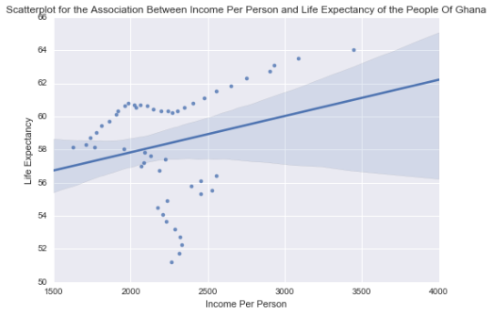
a) q-q plot

The q-q plot was ran to evaluate whether the regression assumption that the estimates from my residuals were normally distributed was met. This is to check if the residual points follow a straight line. That is what I would expect if the residuals were normally distributed.
From the q-q plot image below , it can be seen that, the residuals do not follow a perfect normal distribution which should be a  straight line.

As it does not follow a perfect normal distribution, it indicates that
there might be other variables which will help explain the variability in the
Life Expectancy of the people of Ghana

 

 

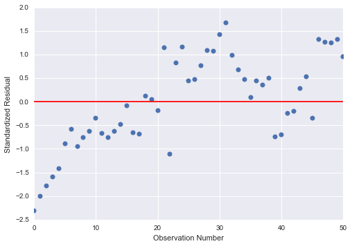
b) standardized residuals for all observations

From the Standardized residuals for all observations it can be seen that
most of the observations fall within +1 and -1 of the Standard Deviation of the
mean. The rest of the residuals fall within 2 standard deviation from the mean
with only 2 residuals which fall beyond -2 standard deviation which is a sign I
might have some outliers but this is a mild one as it is not beyond 3 of the
Standard Deviation. Even these 2 observations are within -2.5 of the standard
deviation. With a standard normal distribution it is expected that 95% of the
residuals fall within 2 standard deviations of the mean. And this is rightly
the case for my standardized residuals.

In determining how well my model fits the observed Ghana population data based
on the distribution of the sample residuals, I did check if more than 5% of the
residuals had absolute values greater than or equal 2 of the standard
deviation, but this was not the case. This means that level of errors in this
model is negligible and accepted; hence the model is a good fit to my observed
data.

This is depicted in the graph below:

s

 

 

REGRESSION PLOTS FOR EXPORTS_C

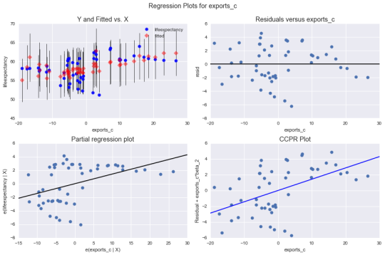
The Residuals versus exports_c graph
(2^nd right in the above 4 set of graphs) shows residuals of each
observation at different values of exports_c .

From the graph it can be seen that the absolute values of the residuals are
higher at lower levels of exports_c,
it gets smaller closer to zero. The values rise again at higer levels of
exports but start to go down lower again. This is consistent amongst all the 4
regression diagnostic plots above. This means that this variable does not
properly predict the lifeexpectancy
of the people of Ghana when there are low or high exports and it is very worse
in this predictions when exports are low. This also might mean I should
consider adding a second order curve polynomial to the exports_c variable in the regression model.

A look at the Partial Regression
plot shows that there is no obvious curve polynomial shape in the exports_c variable. And also all the
residuals are widely spread and far away in a random pattern along a partial
regression line. This indicates a great deal of lifeepectancy prediction error.
Although exports_c shows a
significant association with lifeepectancy
this prediction is weak after controlling for incomeperperson_c and inflation_c.

 

c) leverage plot

This was run to examine observations which might have an unusually large
influence on the estimation of the predicted values of the response variable – lifeepectancy   of the people of Ghana or if there are any outliers
or both.  This is done using the graph
below

 

From the graph above, we can see we have 2 outliers. Although these are
outliers they have small or close to zero values and hence they do not have undue influence on the
estimation of the regression model