Overview

My research work deals with Ghana, a country from the Gapminder
dataset as has already been discussed from the beginning and progression
through this course.

My response variable, lifeexpectancy, is a quantitative response variable that measures the life expectancy of the people of Ghana.

For the purposes of running the Lasso Regression Analysis, I added more variables from the Gapminder website: http://www.gapminder.org/data/
to my original dataset.

The new explanatory variables added are:

male bloodpressure, total population who are females, agricultural
land, aid received, aid received per person, real gdp per capita, female blood
pressure, male body mass index, female body mass index, under five mortality, total fertility rate, cholesterol in men, cholesterol in women, crude birthrate, dead kids per woman, external debt stocks, and energy use

Though all my explanatory variables from the Gapminder website were quantitative variables, in conducting my data management I converted
some of the variables to a 2-level binary categorical explanatory variable in
order to get a proper insight and understanding of lasso regression analysis by
having a mixture of quantitative and categorical predictor variables.

The following are the quantitative explanatory variables which were converted to 2-level binary categorical explanatory variables and their resultant categorical variables

 

Quantitative variable                  Resulting Categorical Variable

incomeperperson                            incomeLevelGrp

exports                                              exportsCatGrp

malebloodpressure                        malebloodpressureGrp

totalpopulationfemale                  totalpopulationfemaleGrp

A lasso regression analysis was conducted to identify a subset of variables from a group of 22 categorical and quantitative predictor variables that best predicted a quantitative response variable measuring life expectancy of the people of Ghana. The categorical predictors included were the ones above-stated (which I converted from quantitative to categorical). The full list of quantitative explanatory variables included is, inflation, democracy score,
agriculture, agricultural land, aid received, aid received per person, real gdp
per capita, female blood pressure, male body mass index, female body mass index, under five mortality, total fertility rate, cholesterol in men, cholesterol in
women, crude birthrate, dead kids per woman, external debt stocks, and energy use

The data were randomly split into a training set that had 70% of the observations and a test set that catered for 30% of the observation. The least angle regression algorithm with k=10 fold cross validation was used to estimate the lasso regression model in the training set, and the model was validated using the test set. No precomputed matrix was used. The change in the cross validation
average (mean) squared error at each step was used to identify the best subset
of predictor variables.

Some of my variables shrank towards zero during the lasso regression analysis. This allowed for better interpretation of my model and helped identified variables which most associated with my response variable.

Since the penalty term in Lasso Regression is not fair if the predictor variables are not on the scale meaning, not all the predictors get the same penalty, I standardised all my predictors to have a mean = 0 and standard deviation of 1 including my binary predictor variables which eventually put all the predictors on the same scale.

I printed my predictor variables and the associated co-efficients.
The predictors with regression coefficient that do not have a value of zero (0)
were included my selected module. Predictors with regression co-efficients
equal to zero (0) means that co-efficient for those variables were shrank to
zero after applying lasso regression penalty and they were subsequently removed from model.

These were

cholesterolinmen’: 0.0,

‘cholesterolinwomen’: 0.0,

‘crudebirthrate’: 0.0,

‘energyuse’: 0.0,

exportsCatGrp’: 0.0,

‘femalebloodpressure’: 0.0,

‘femalebodymassindex’: 0.0,

‘incomeLevelGrp’: 0.0,

malebodymassindex’: 0.0,

totalfertilityrate’: 0.0,

‘totalpopulationfemaleGrp’: 0.0,

‘underfivemortality’: 0.0}

In total 12 predictor variables were removed from my model and 10 variables were retained out of the 22 overall quantitative and categorical variables.

Variables which were retained in my analysis can be seen
below:

Since I standardized the variables to be on the same scale, I
can also use the regression co-efficients to determine which variables are
strongly associated with life expectancy of the Ghanaian population

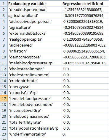
Sorting my regression my coefficients I can see that ‘deadkidsperwoman’ which has a co-efficient of  -1.2592958215300067,  is strongly associated with the life expectancy of the people of Ghana. This is is followed by agriculturalland with a coefficient of  -0.50919770050676894, and then ‘aidreceivedperperson’ with
a coefficient of  0.32008602261819619,

The full list of the variables and the strength of association with life expectancy of the people of Ghana can be seen in this image below. (variables
with zero coefficients were removed from the model)

 

 

deadkidsperwoman, agriculturalland, agriculture, externaldebtstocks, aidreceived, democracyscore, malebloodpressureGrp were negatively associated with life expectancy of the people of Ghana whereas aidreceivedperperson, realgdppercapita, inflation, were positively associated with the life expectancy of the people of Ghana.

Also progression plots were created to visualise the results.

This plots shows relative importance of the predictors selected at any step of the selection process however the regression coefficient changes with the addition of each variable at each step of the process.

As noted from the regression co-efficients, ‘deadkidsperwoman’
with the highest regression co-efficient was entered first with the yellow line,
followed by agriculturalland which are both negative and then followed by ‘aidreceivedperperson’ which is a positive coefficient

A plot to show the mean squared errors on each fold was generated

 

From the mean squared error plot, I can see there is variability across the individual cross validation folds in the training data set but the change in the mean square error as variables are added to model follow almost similar pattern. Initially it decreases rapidly and it turns to fluctuate just before and after the alpha line and gets to a point where adding more variables do not result in much
reduction in the mean squared error.

Printing the average Mean squared errors and also the R-square from both the training and test data sets, I get the following results.

training data MSE

0.00998814282209

test data MSE

0.102424584365

training data R-square

0.994366415288

test data R-square

0.843994145664

From the R-squared values, it can be interpreted that the selected model explains 0.994366415288

(99.4%) of the variance of life expectancy for training dataset and 0.843994145664 (84.4%) of the variance of life expectancy of the people of Ghana in test dataset

 

####################################

PYTHON CODE

####################################